Introduction Case Organization Design Variables & Constraints Search Engines (Multilevel) Evaluation Scripts Parallel Evaluations Run & Results Results Desktop

Search Engines (Multilevel) In the Search Engines (Multilevel) tab the user sets the number of optimization levels, their type (Evolutionary Algorithm, Steepest Descent/Conjugate Gradient, SQP) and configures the tuning parameters of each level. The configuration of each level appears after selecting it from the pull-down menu evolution features. Search Engine: Evolutionary Algorithm Evolutionary algorithms have been traditionally used in EASY as search engine. The tuning parameters allow the user to select a conventional EA, its distributed variant DEA, MAEA or DMAEA. All parameters are included in seven tabs (General, Hierarchical, Distributed, Convergence, Population, Operators and IPE). To use evolutionary algorithms at any Search level, the EA tab should be checked. General (Settings) The General (settings) tab allows the user to configure all the settings of the EA that do not fall into any other category. 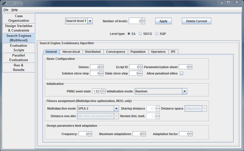The tab is split in four sub-panels: Basic Configuration Initialization Fitness assignment (MOO) Design parameters limit adaptation In the Basic Configuration panel the user defines the number of Demes that will evolve in this level and the Script ID (with the same numbering as in the Evaluations Scripts tab) that will be used. The solution is exported in the solution file for a generation step defined in Solution store step box. The state file, needed in case of continuation, is updated according to the State store step box. The second panel is related to the algorithm's Initialization. The Pseudo Random Number Generator seed is used to initialize the random number generator. Changing the seed produces a different sequence of (pseudo) random numbers that affects the evolution and, therefore, the final solution. The combo box Initialization mode, apart from the default random initialization, allows the initialization of the population from an ASCII file. The Fitness assignment (MOO) panel is enabled only when dealing with MOO problems and contains some extra settings that have to be specified. The most critical of them is the Multiobjective Mode which determines the way fitness score is assigned to the individuals depending on the each objective score. The available options are: Front Ranking The fitness of each individual is equal to the number of front it belongs. Sharing (NSGA) Like front Ranking but within each front the fitness score is differentiated depending on the number of individuals in the neighbourhood forcing the Pareto front to spread in the objective's space. In this case extra parameters may be set. Sharing distance is a nondimensional number determining how close the individuals may be to penalize their fitness score. A value of 0.01 is recommended. The higher the value the more Pareto front is expected to spread out, in the expense of worsening its position. Distances are recommended to be counted in the objectives space which is the space of interest as the results are displayed there and typically it has a smaller dimension. Nested space is a fictitious space that takes into account distances in both the variables and objectives space. The distances in the objectives space are multiplied with the value specified in the Nested distance multiplier box. Distances are recommended to be non-dimensionalized with the Min-Max objective or variable of the current front. SPEA 1 Strength Pareto Evolutionary Algorithm. The fitness score of an individual depends on the number of individuals it dominates. SPEA 2 Strength Pareto Evolutionary Algorithm 2. The fitness score still depends on the number of individuals dominated but a different algorithm is used. Additional the number of individuals in a neighbourhood is taken under consideration during fitness score assignment to encourage Pareto front spreading on the objective's space. SPEA 1.5 A SPEA implementation which uses for fitness assignment SPEA 2 algorithm without the part which encourages front spreading. The Limits adaptation panel allows variables to get out of the limits defined in the table in the Desing Variables & Constraints tab by internally adjusting them. The user selects the Frequency (in generations) to perform limits adaptation. The Maximum Adaptations box specifies the maximum allowed number of limit adaptations. Set it to zero to disable limit adaptation. Each time a limits adaptation occurs, the variables range (upper - lower limit) is multiplied by the factor defined in the Adaptation Factor box. It should be less than 1 to decrease variables range and increase accuracy. Recommended values are about 0.8. Hierarchical In an Hierarchical EA, a low-accuracy, low-cost model is used to evaluate the populations of an EA, which may therefore explore the search space at low CPU cost. In the same time, a second EA, which implements a computationally more expensive tool with higher modelling accuracy, is fed by the elite solutions identified by the former EA and continues the search for the optimal solution. The high-level EA uses smaller populations, in order to keep the cost as low as possible. 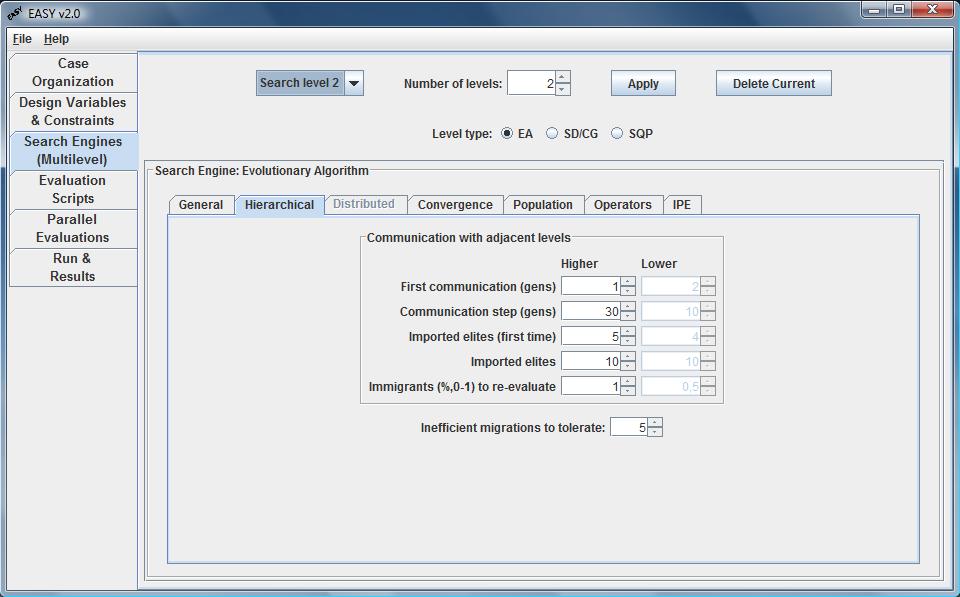In this tab all parameters regarding the communication between adjacent levels (higher and lower) are configured. The user defines the generation to initiate the communication (First communication) as well as the frequency of communication (Communication step) in terms of generations. The number of Imported elite individuals (for the first and the subsequent communications) ia also defined. Some of them are re-evaluated, according to a percentage of Immigrants to re-evaluate, while the rest keep their low-cost evaluated fitness. Finally, in the Inefficient migrations to tolerate combo box the maximun number of inefficient migrations allowed in=s defined. Thus, the evolution of lower levels can be terminated if they fail to update the higher level above this threshold. Distributed Distributed EAs (DEA) subdivide the entire population in smaller ones, called islands or demes, and evolve them in semi-isolation by regularly exchanging the most promising among their population members. It has clearly been proved that DEAs outperform conventional EAs. 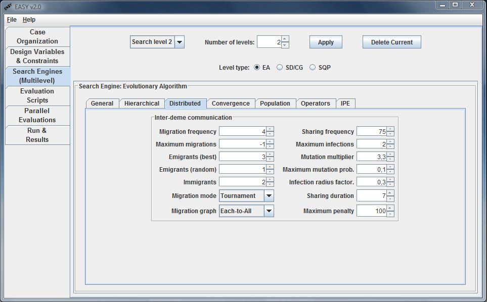Through this tab, the user handles DEA features. Once the number of demes on General tab is more than one, the Distributed panel with the demes communication settings is activated. The user is able to select the frequency, in terms of generations’ steps, when migration and infection occur between the demes, as well as the number of maximum migrations to perform. If the last one is set up to -1, infinite number of migrations is allowed. The minimum number of elite and random immigrants is also defined. The migration mode combo box defines if the immigrants will replace individuals in other demes randomly, by means of fitness value (tournament where the worst individuals are being replaced) or both. 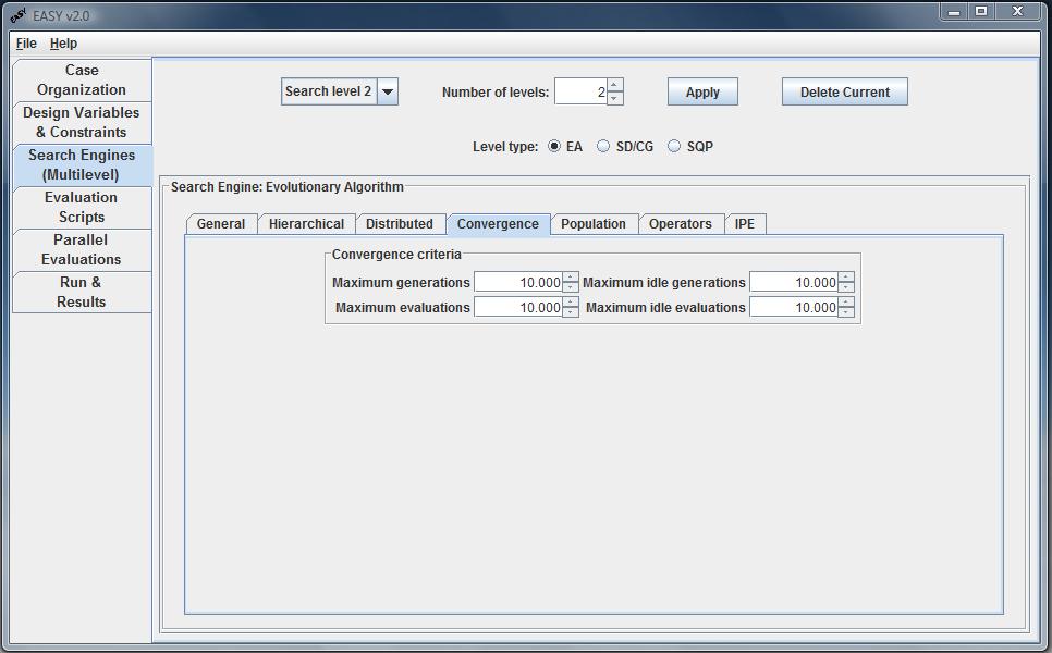Convergence EASY stops the evolution when one of the Convergence Criteria is met. This may be an upper limit to the number of evaluations or generations, or an upper limit in the number of idle evaluation or generations. An evaluation or generation is considered as idle if no better solution is found. Population This tab is responsible for setting offspring, parent and elite population sizes, elitism and parent selection operators. 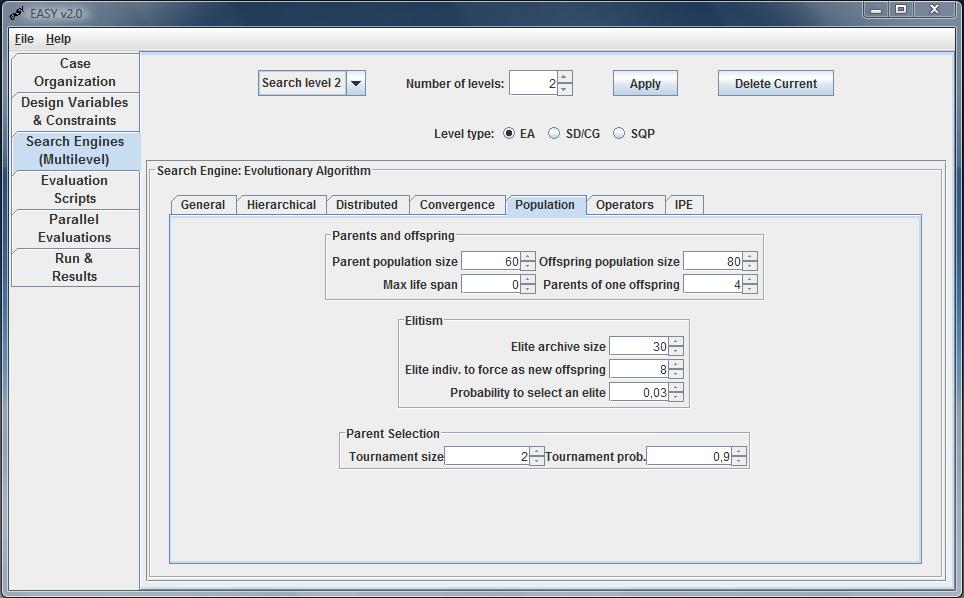The user defines the population size of parents and offspring. Recommended ratio between parents and offspring population is about 1/3...1/7 depending on the desired selection pressure. Maximum life span is the maximum number of generations a parent is allowed to withstand. The user may also specify the number of parents that form one offspring. A typical setting for a genetic algorithm is two parents per individual. A greater number of parents per individual (3-5) is reported to give a better convergence rate. A pool of elite individuals is kept which, at any moment, corresponds to the optimal solution to the problem. In single objective optimization, the pool consists of the best individuals encountered during the evolution while in multi-objective optimization this is the maximum number of Pareto front entries. In the Elitism sub-panel the Elite archive size is selected. The pool of elit individuals may be used to forcibly copy some of them to the current offspring population replacing the worst offspring. A value of 1-2 individuals is recommended for the corresponding box. Additionally a random elite individual may be selected as a parent with a probability specified in the corresponding box (values about 0.01 - 0.1 (1% - 10%) are recommended). If the parents population size is close or equal to the offspring population size then the parent selection operator must be active, that is the number of tournament size must be greater than 1 which corresponds to a random selection operator. Using the tournament selection a parent is the winner of a tournament between other parents whose number is specified in the corresponding box. A recommended value is 2-3. Parents compete with their fitness score. The probability for the parent with the best fitness to win is recommended to be in the range of 0.8-1. Operators This tab sets the variable coding scheme and parameters for crossover and mutation operators. Please refer to the relevant subsection for the coding of your choice for more information on mutation and recombination operators. 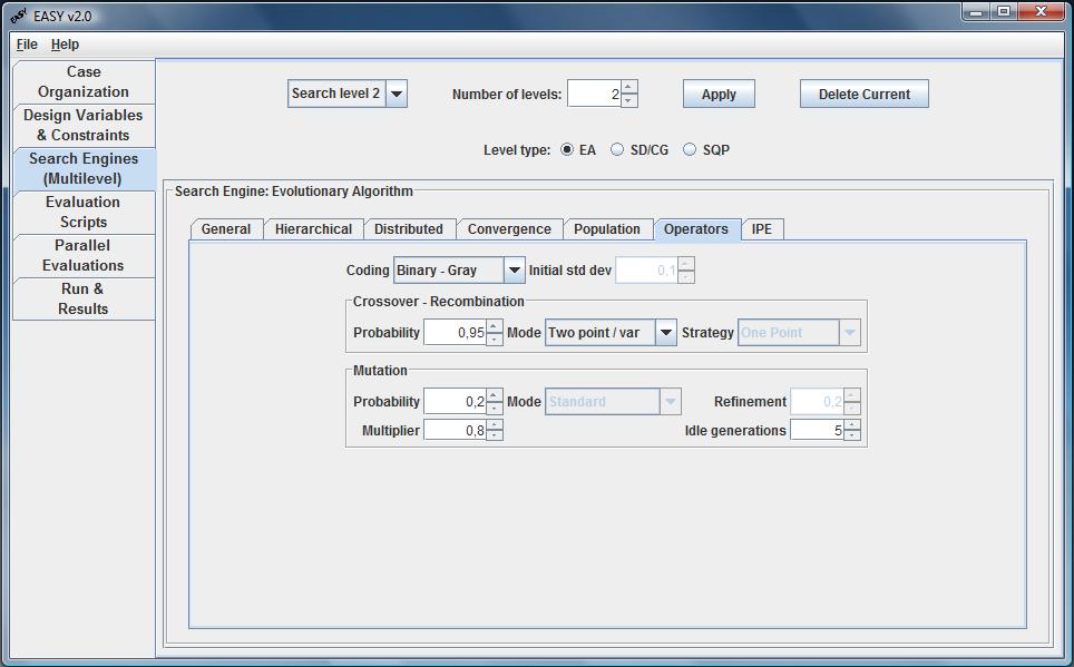Coding combo box Binary Any individual is represented by a string of binary digits (bits), whose number is equal to the sum of bits for each variable, as defined in the variables tab. The range between Min and Max is discretized in 2^b intervals, therefore the minimum step size of a variable is (Max-Min)/(2^b-1). By increasing b, the problem complexity increases too but also increases the expected computing accuracy for each variable. Binary - Gray It is likely that, using binary coding, the representation of two successive numbers (such as 011111 and 100000) may differ in many bits. Gray coding uses an additional transformation to ensure that the representation of two successive numbers differs only by one bit. Often this technique increases the convergence rate of the algorithm which means that less evaluation calls are needed for obtaining comparable results. Real The representation of an individual is just the vector containing the real values of its variables. The accuracy of each variable is equal to the one supported by the operating system (as good as possible). Since the search space is expanded more evaluations may be needed. Recombination and mutation performed to each individual depend on the coding selected. Real with Strategy The representation of an individual is a vector containing the real values of its variables plus a list of strategy parameters, i.e. parameters which affect the recombination and mutation operators. Including strategy parameters in the representation may increase the convergence rate but the optimization process may be more susceptible to premature convergence. Initial std dev Initial standard deviation. This box is enabled only if the Real with strategy coding scheme is selected. It is a measure of the initial step size of the variables in the search space. For inexperienced users, the value 0.01 (1%) is recommended. Crossover-Recombination The crossover (genetic algorithms terminology) or recombination (evolutionary terminology) operator produces new individuals by combining the information contained in the parents. This operator applies with a probability defined in the Probability box. The recommended value is close to 0.9 (90%). Depending on the coding of the variables the following operators can be applied: Binary coding (with or without Gray coding) One point: The binary string is cut at a random point. The sub-strings are exchanged between the parents. If each offspring is the outcome of two parents: If each offspring is the outcome of three parents: Two point: The binary string is cut at two random points. One point / var: The binary string is cut at a random point, separately, for each one of the variables. Discrete: Substrings that constitute an entire variable are exchanged. Uniform: A random binary mask is generated of size equal to the number of bits per individual. The binary string of the new offspring is created by copying the bits of the parents depending on the value of the mask (0 or 1) at each position of the binary string. Two point /var: The binary string is cut at two random points for each optimization variable. Real coding (with or without strategy parameters) One point: Like the one of binary coding but extended to real coding. In the above example the random cut point is variable number 4 and r is a random number. Two point: Two random cut point are selected and the recombination is performed as in the case of one point. G. Intermediate: Variable values of the offspring are chosen between the variable values of the parents. Recombination for each variable is performed as Discrete: This operator performs an exchange of variable values between the individuals. Each variable is randomly selected from a parent and copied without further modifications. No averaging: This operator acts like the generalized intermediate but the random number r is substituted by Clearly C does not belong in [0,1] thus the averaging effect in avoided. Intermediate: Like generalized intermediate but r is always equal to 0.5. Simulated bin: Using this operator points near parents are more likely to be selected. Offspring = 0.5[(1+b)Parent1+(1-b)Parent2], where b = (2u)^(1/(n+1)), if u less 0.5 or b = (1/(2(1-u)))^(1/(n+1)), otherwise. u in [0,1], n in N (great=0), here n=1. In case of Real coding applied also to the strategy parameters, the same recombination operators are available for the strategy parameters. Generalized intermediate is recommended for the strategy parameters. Mutation After recombination, every offspring undergoes mutation. The mutation operator explores the search space by introducing new genetic material in the population. Offspring variables are mutated by small perturbations, with low probability. The variables coding determines the operator used: Binary coding (with or without Gray coding) Mutation probability is the probability of mutating a bit in the binary string (changing from 0 to 1 or vice-versa) and is generally set to be inversely proportional to the sum of bits of an individual. Thus for binary coding a mutation rate of (1...3)/bits_total is recommended. Idle generations: Number of successive generations that no better solution has been found. If this number is exceeded then the mutation probability is multiplied by the factor defined in the multiplier box. Real coding The mutation probability is the probability used to mutate any variable of an individual. Refinement: Parameter active only in real coding that determines how much a variable will change if it is mutated. Greater values lead to great changes. A value of about 0.2 is recommended. The number of idle generations and the multiplier have the same meaning. Real coding with strategy parameters: In evolutionary strategies where this coding is used mutation of the variables and strategy parameters is performed in a way that mutation probability is not used and thus, it is disabled along with idle generations and the multiplier that control it. The standard mutation operator may be changed and use instead of it a step size control mechanism. Inexact Pre-Evaluation EASY offers the opportunity to use Artificial Neural Networks as a low-cost Inexact Pre-Evaluation (IPE) Tool, in order to reduce the number of calls to the exact evaluation tool. The configuration of IPE is split in two panels. 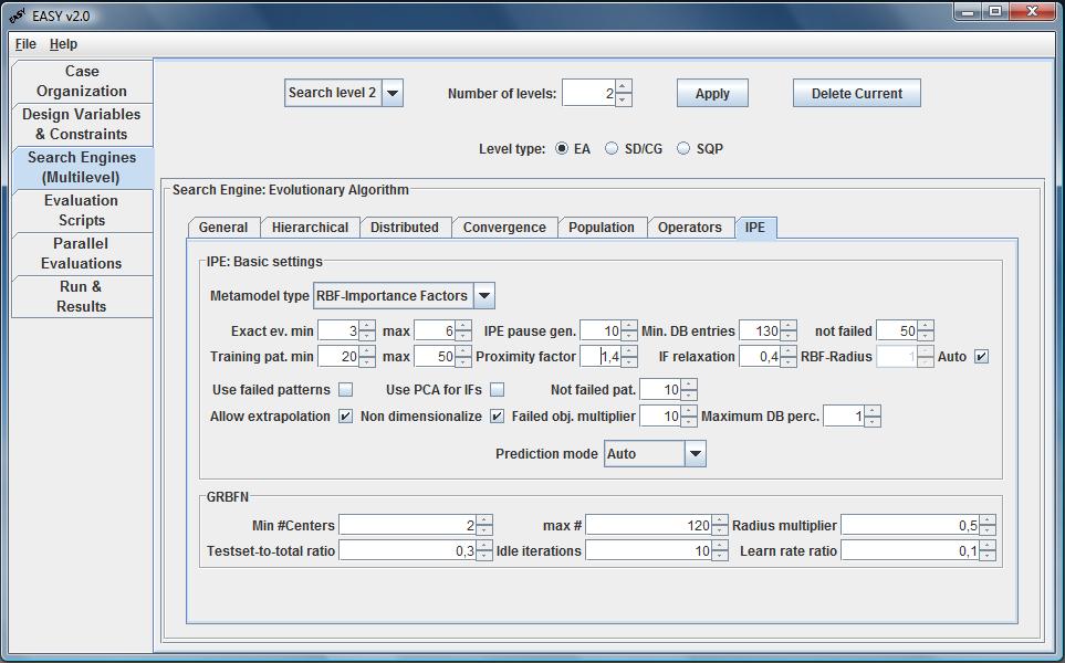IPE: Basic settings In the Metamodel type combo box the user selects the metamodel to use (None, RBF, RBF with Importance Factors, External). Once, a metamodel is selected, a number of parameteres should also defined. The minimum number of exact evaluations per generation should be less than the size of offspring population. A value of 1-5 is recommended. In case of sticking on local optima for several generations, IPE is paused and re-enabled again, filling the database with new exactly evaluated patterns. The Min. DB entries define the minimum exact evaluations to be performed before starting IPE. The last one is recommended to be greater than 100. The minimum number of training patterns is recommended to be in the range of [8, 20] while the maximum in the range of [12, 30]. The proximity factor determines the exact number of training patterns used for the training of the network. The higher the value the more close the training patterns will be to the maximum allowed. A value of about 1.2 is recommended. Extrapolation of objectives outside the bounds defined by the training set is generally not recommended. The Non-Dim checkbox is recommended to be checked to ensure that the individual that will be predicted is always between [0,1] after nondimensionalization. If failed individuals are selected for the training of the network their fitness score will be the one of the worse selected individual multiplied by the number specified in the corresponding box. A value of about 10 is recommended. The use of importance factors improves the prediction capabilities of the network, particularly in single objective optimization. Importance factors are updated with a relaxation which is recommended to be about 0.5. GRBFN Growing Radial Basis Function Networks are used when the heuristics suggest that the neural networks are extrapolating and extrapolation is allowed. In extrapolation mode the radial basis function centers are computed using an iterative procedure in which the training patterns are divided into training and test set using a user-defined ratio. The algorithm iterates until a user-defined number of idle iterations occur. The user also define the number of centers (min,max) to use for RBF networks, a Radius multiplier to multiply the heuristics radius, a Testset-to-total ratio i.e. the percentage of the patterns to use as testing set and a Learn rate ratio. 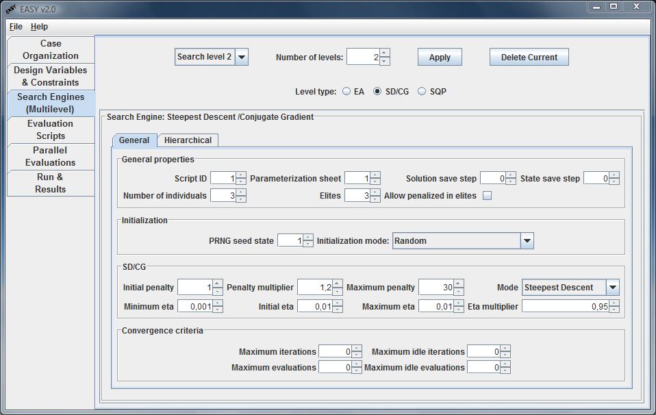Search Engine: Steepest Descent/Conjugate Gradient The second search engine implemented in EASY is steepest descent/conjugate gradient. This search mode is configured in the general tab (hierarchical tab has the same parameters with EA search engine and will not be discussed). The general tab is subdived in four panels: General properties Initialization SD/CG Convergence criteria Panels for General properties, Initialization and Convergence criteria (corresponds to Convergence tab in the EA search engine) have already been discussed. In the SD/CG panel, the user may define the descend mode among steepest descent, conjugate gradient (Fletcher-Reeves variant) and conjugate gradient (Polak-Ribiere variant) in the Mode combo box. In this sub-panel, further details conserning the eta value (minimum, maximum, initial and multiplier) and penalty (initial, maximum and multiplier) are also defined. Search Engine: Sequential Quadratic Programming The third search engine implemented in EASY is the SQP method. Main parameters are same as in EA and SD/CG search engines, apart from the SQP sub-panel in the general tab. In this sub-panel, the user defines the Hessian apprx (BFGS or Damped BFGS), the trust region radius (min, max, initial), the eta and the penalty (initial, maximum and multiplier). Finally, an option to restart SQP in case of poor predictions is available.